Singularity is a relatively new tool that extends docker-style containerized compute into the hands of researchers on compute clusters. For security reasons, most compute clusters did not allow docker containers, and would require any software to be installed by system administrators. However, singularity resolves the security challenges of docker and have taken over the primary method of creating portable software. Container-based software really make research software reproducible across different labs/compute environments because it can function as an easy distribution means for software. This is because the original developer can define every installation step in a platform-independent method. Once built, anyone that wants to test the software can download the container and run the software. Not all containers are equal, though. There are many flavors of linux that you can start with, each with their own advantages and disadvantages that can influence how efficient your software performs. We do a lot of compute on our large datasets, and squeezing out extra performance from these singularity images can mean the difference in compute time of weeks. It is important to benchmark the performance of software you design.

For this benchmark, I’m going to be testing 3 types of operations in python: reading in data, basic calculations on data, and large-scale multiplications on data. I’m also testing across multiple base images, including Alpine-linux and Debian Buster (python 3.6 and python 3.8). The major reason I’m comparing Alpine and Debian Buster is because Alpine uses musl as its c library while Debian Buster uses the much more traditional glibc c library.

Reading in data is usually a fairly straight forward operation and depending on the size of the dataset can take some time. Normally one would expect the bottleneck of reading data to be on the physical disk IO, but here we see that the alpine image takes 80% of the time that the debian variants do.

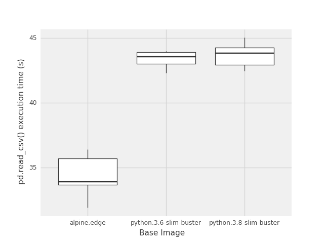
Reading Data Results

Basic calculations are also a common operation within data analysis. Again, we observe alpine is outperforming debian images, but this time alpine takes 60% of the time that buster images do!

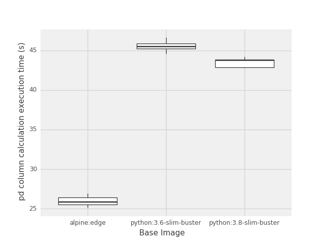
Column Calculation Results

Finally, the vast majority of the compute that I was running this benchmark for is based on running continuous wavelet transforms on the data. This is often a very compute-intensive calculation and we want to pass a lot of data through it. Very surprisingly, the faster image reverses and is now the debian buster image with the latest version of python. Even more surprising is that it takes 60% of the time to calculate it compared to the alpine image.

CWT Results

If you have a lot of compute that you’re planning on doing, it is often worth running benchmarks on different things you can change with the environment. In this case, choosing the wrong starting image would have changed 9 days worth of cluster compute into 15 days worth of compute. If you’re using singularity and happen to have large datasets that take multiple days to compute, it is probably worthwhile to trial different base images to see if you can squeeze out some extra efficiency.

Extra fun details for the benchmarks:

• Compute cluster environment was tested on a Supermicro BigTwin server node with 72 cores at 2.7GHz and 768 GB of DDR4 RAM.
• The benchmark process only used 2 CPU cores and 4GB RAM, so the nodes were sometimes shared with other compute jobs (although they didn’t influence the results).
• Data reading showed no difference between a local solid state drive and the cluster’s network Data Direct Networks Gridscalar GS7k GPFS (general parallel file system).
• Python library versions were controlled for, so all comparisons were all running the same versions. They were using similar but not exactly the same libraries that they were compiled against (gfortran was newer in alpine:edge).
• Plots were made in python using plotnine, which is a ggplot plotting grammar frontend for matplotlib in python. If you like ggplot and python, I’d recommend you check it out.