Multivariate response data are routinely generated from experiments carried out in our lab. For example, several interrelated gait metrics such as stride length, step length, limb duty factor etc. are extracted from each stride of the mouse. The goal is to gain insights on the gait defects in mice using these metrics. We want to explore how variables such as body length, genotype and sex of the mouse affect gait.
A multivariate linear model (MvLM) is an extension of the univariate linear model for regression and ANOVA. It allows us to characterize and quantify the effect of covariates (body length, genotype etc.) on two or more response variables (gait metrics) simultaneously. Statistical hypothesis tests for MvLMs closely parallel the familiar F and t-tests for univariate models and serve as an appealing alternative to running several univariate tests separately. However, multivariate analyses are more complicated than univariate approaches, especially when it comes to understanding and communicating results about the effects of covariates and model parameters.
HE plots provide a compact visual summary and aid in simple interpretation of MvLMs which may not be readily achieved at a glance. The essential idea behind the Hypothesis-Error (HE) plots is that any multivariate hypothesis test can be represented visually by an ellipsoid (or ellipse in 2D or a line in 1D) by superposing an H ellipsoid representing variation against a null hypothesis on an E, representing error variation. The HE plots provide a visual test of significance signaled by the H ellipsoid projecting outside that of E as demonstrated by illustrative examples below. See Friendly et al. (2013) for a detailed discussion on the role of ellipsoids in statistical data visualization. The plots are implemented in two and three dimensions in the heplots package in R.
Example 1
Consider the data frame Sod giving data on stride length, step length and limb duty factor measures of the gait metric at two distinct test ages for 32 mice who were observed in one of two groups: Controls and Mutants. Our repeated measures data, therefore, has two between-subject factors (Genotype & Sex) and one within-subject factor (TestAge).
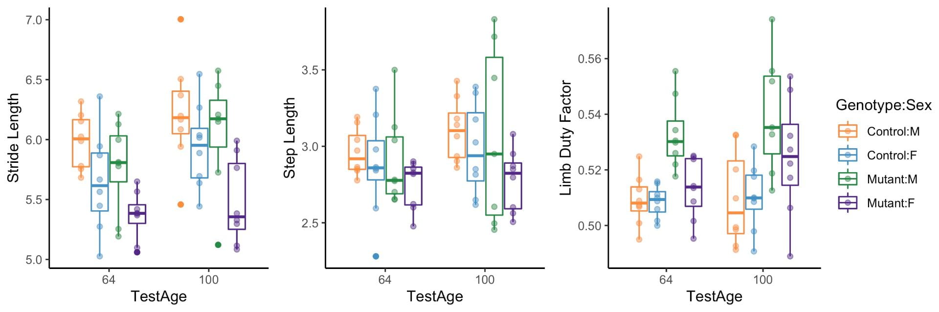
Figure 1. Boxplots of the gait metrics give an initial view of the data.
We perform a multivariate analysis of covariance (MANCOVA) where the focus is on differences among groups (controls vs mutants) defined by the factor Genotype, adjusting for the quantitative covariate BodyLength. The results from multivariate tests for all between- and within- effects obtained from fitting a multivariate linear model are displayed below.
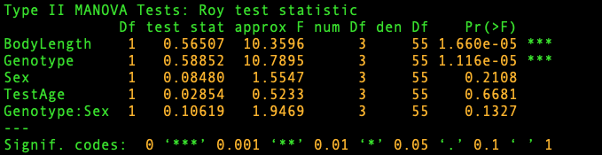
Next we will see how HE plots provide a compact visual summary of an MvLM mirroring the tabular representation from above and, at the same time, reveal the nature of these effects. For this example, all ellipses for the main effects plot as degenerate lines because all effects have 1 degrees of freedom (see the output above).

Figure 2. HE plot for the multivariate linear model showing between-subject effects in the space of limb duty factor and stride length variables.
- The fact that the H ellipse for the Genotype effect (black line) extends outside the E ellipse signals that this null hypothesis is clearly rejected. In other words, the Controls have higher stride length and lower limb duty factor compared to Mutants and these differences are not due to chance alone.
- The effect of Sex is not significant, but the HE plot shows that males have higher stride lengths than females. Likewise, the TestAge and Genotype:Sex (interaction) effects fail significance and the observed differences are due to chance.
- Since BodyLength is orthogonal (perpendicular) to y-axis, BodyLength has zero effect on Limb Duty Factor.
Example 2
Consider the data frame Mecp2 giving data on stride length, step length and limb duty factor measures on the gait metric at two distinct test ages of 32 mice who were observed in one of the three groups: Controls, Hemis and Hets. For Mecp2, there is a perfect association between the two between-subject factors Genotype and Sex. In other words, all Hets are females and all Hemis are males.
The results from MANCOVA analysis and the corresponding HE plots are displayed below. Note that the H ellipse for the main effect Genotype is actually an ellipse since Genotype has 2 degrees of freedom. The ellipse for the main effect BodyLength degenerates to a line since it has 1 degree of freedom.

.
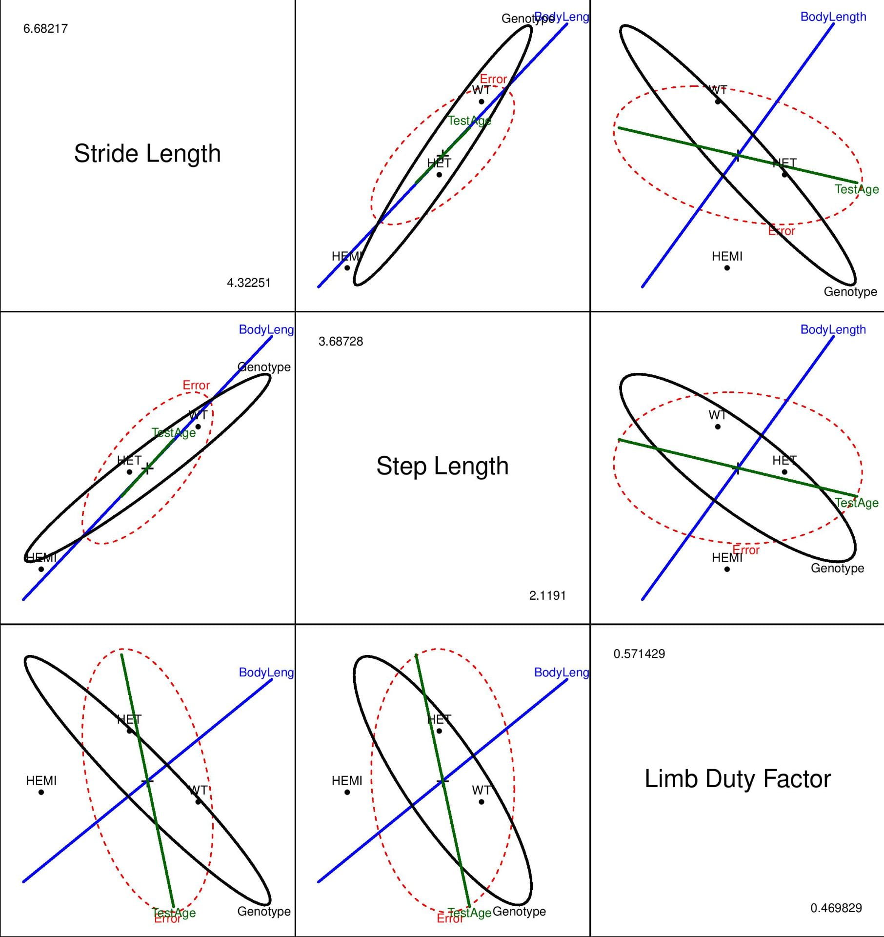
Figure 3. HE plot for the multivariate linear model showing between-subject effects for all pairs of gait variables. For example, the plot in row 2, column 1 shows the between-subject effects in the space of stride length and step length.
Before we interpret the plots in the grid above, one should note that the grid is ‘symmetric’ i.e. the plots in panels (row 2, column 1) and (row 1, column 2) are identical in that they convey the same information. Henceforth, (a, b) refers to the plot in row a and column b.
- The fact that the H ellipse for the Genotype effect (black ellipse) extends outside the E ellipse in all plots provides strong evidence against the null hypothesis. Moreover, from (1,2), we can conclude that the control mice (WT) have higher stride lengths and step lengths than both Het and Hemi mice. Similarly, from (3,1) we can see the Hets have a higher limb duty factor compared to both Hemis and controls (both of which have roughly equal limb duty factors).
- We see that the ellipse (green line) for the main effect TestAge almost touches the error ellipse in all plots with limb duty factor as one of the variables which indicates that TestAge might be ‘significant’ for limb duty factor.
- The positive slope (orientation) of BodyLength (blue line) implies that mice with larger body sizes have larger stride lengths, step lengths and limb duty factors (as expected).
- The size and orientation of the ellipses for the error and main effects provide other useful information about model fits. For example, comparing (2,1) and (2,3), we see that the error ellipse is slightly ‘bigger’ for (2,3) which implies that the main effects explain more variability in stride length and step length than they do in limb duty factor.
The geometry of HE plots provides a visual mean of judging both effect size and significance. Here the emphasis is not on simplistic p−values for significance testing, but rather on visual assessment of the strength of evidence against a null hypothesis and how this relates to the response variables shown.